End to end ML Retail Forecasting

A comprehensive Machine Learning pipeline to forecast sales for 50 items across 10 stores over a 3-month period. It covers the end-to-end workflow, from data analysis and feature engineering to model tuning and interpretation, structured for reproducibility and deployment.

Table of Contents

1. Business Problem & Objectives
2. Tech Stack
3. Project Structure
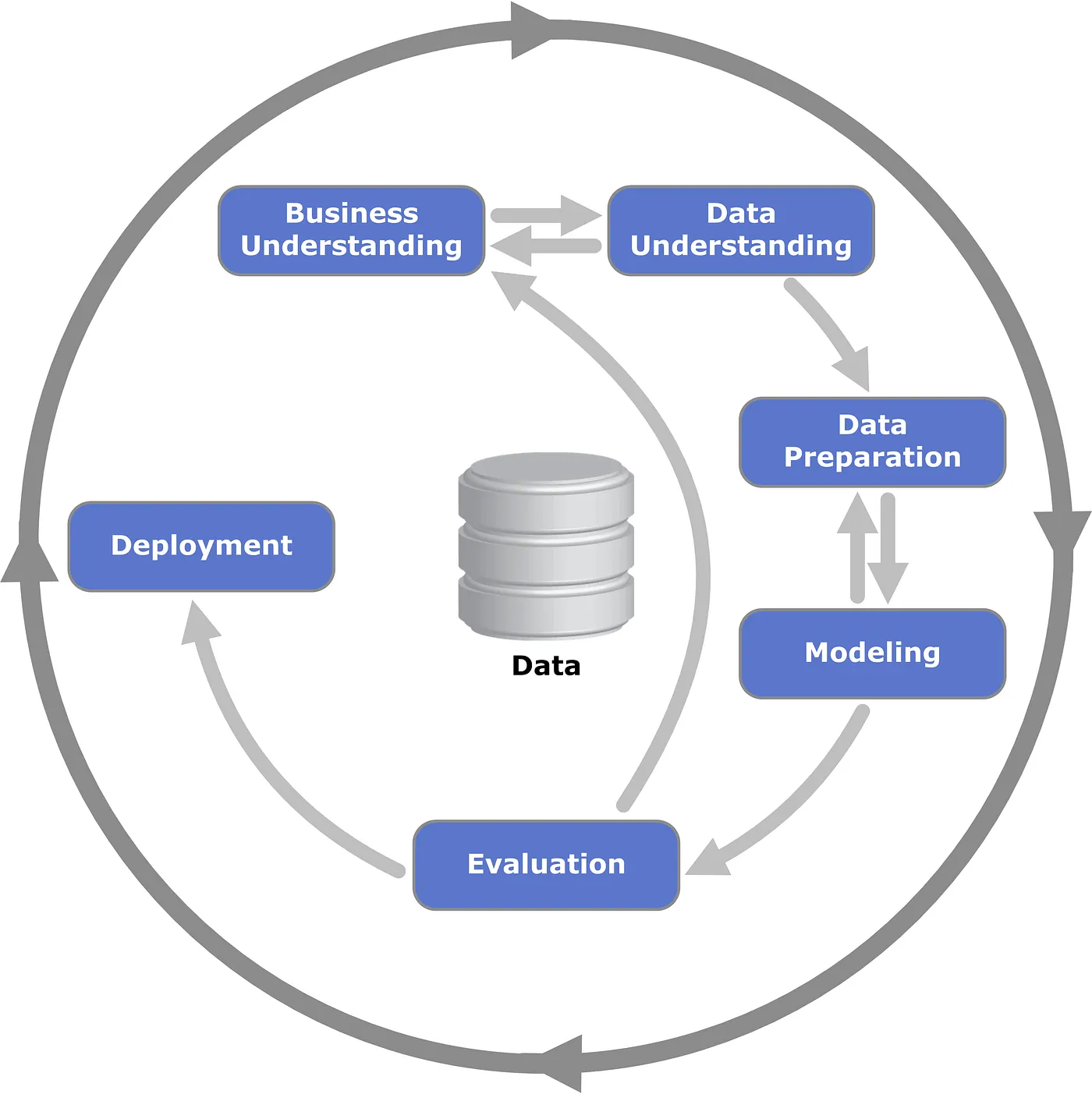
4. Methodology: The CRISP-DM Framework
5. Exploratory Data Analysis (EDA) & Key Insights
6. Modeling Pipeline
7. Model Evaluation & Interpretation
8. Business Impact: The Financial Forecast
9. Getting Started: Running the Project Locally
10. Dataset

Business Problem & Objectives

A retail company needs to optimize its inventory management and investment strategy across 10 stores and 50 different products. Inaccurate sales predictions can lead to stockouts (lost sales) or overstocking (increased holding costs).

The primary objectives of this project are:

• Uncover Insights: Analyze 5 years of historical sales data to identify key trends, seasonal patterns, and sales drivers.
• Build a Predictive Model: Develop a robust machine learning model to accurately forecast sales for each item-store combination for the next 3 months.
• Deliver Actionable Forecasts: Translate model predictions into a clear financial forecast, including best/worst-case scenarios, to support strategic business planning.

Tech Stack

• Programming Language: Python 3.11
• Data Manipulation & Analysis: Pandas, NumPy
• Data Visualization: Matplotlib, Seaborn
• Statistical Modeling: Statsmodels (for time series decomposition)
• Machine Learning: Scikit-Learn, LightGBM
• Hyperparameter Tuning: Optuna

Project Structure

The project is organized as a Python package, ensuring modularity and reproducibility.

├── input/                  # Stores raw data files (train.csv, test.csv, etc.)
├── models/                 # Stores serialized model files (.pkl)
├── notebooks/              # Contains EDA and Modeling Jupyter notebooks
├── reports/                # Stores generated plots and images for documentation
├── src/                    # Source code for the project
│   ├── artifacts_utils.py  # Utility functions for saving/loading artifacts
│   ├── modelling_utils.py  # Core modeling and feature engineering functions
│   └── exception.py        # Custom exception handling
├── .gitignore              # Specifies files to be ignored by Git
├── README.md               # Project documentation (you are here!)
├── requirements.txt        # Lists all project dependencies for easy installation
└── setup.py                # Makes the project installable as a package

Methodology: The CRISP-DM Framework

We follow the Cross-Industry Standard Process for Data Mining (CRISP-DM) to ensure a structured and iterative approach.

1. Business Understanding: Defined project objectives and success criteria.
2. Data Understanding: Initial data exploration and quality assessment.
3. Data Preparation: Feature engineering, transformations, and splitting.
4. Modeling: Model selection, training, and hyperparameter tuning.
5. Evaluation: Assessed model performance against business objectives.
6. Deployment: Out of scope

Exploratory Data Analysis (EDA) & Key Insights

• Overall Trend: Sales show a consistent upward trend over the 5-year period.
• Seasonality: Sales peak annually around July and dip at the beginning of the year.
• Weekly Pattern: Sales build throughout the week, with Sunday being the highest sales day.
• Store Performance: Stores 2 and 8 are top performers, while stores 5, 6, and 7 lag behind.
• Product Performance: Items 15 and 28 are the consistent best-sellers.

Figure 1: Overall sales show a clear upward trend and strong seasonality.

Figure 2: Sales distribution highlights top and bottom-performing stores.

Modeling Pipeline

1. Time Series Decomposition & Preprocessing

The time series was decomposed into trend, seasonal, and residual components using statsmodels to confirm patterns identified in the EDA. To stabilize variance and handle the right-skewed nature of the sales data, a log-transformation was applied to the target variable (sales), which significantly improved model performance.

Figure 3: Log-transforming the target variable creates a more normal distribution.

2. Feature Engineering

A rich set of features was created to capture the temporal dynamics of the data:

• Date-Based Features: month, dayofweek, dayofyear, weekofyear.
• Lag Features: Sales from previous periods (e.g., 91 days, 364 days ago) to capture auto-correlation.
• Rolling Window Features: Rolling means and standard deviations (e.g., 1-year rolling average) to smooth out noise and capture trends.
• Exponentially Weighted Mean (EWM) Features: To give more weight to recent observations.

3. Validation Strategy

• Time Series Split: The data was split chronologically, using the last 3 months for the final test set to simulate a real-world forecasting scenario.
• Time Series Cross-Validation: A TimeSeriesSplit with a 3-month validation window and a 1-week gap (to prevent data leakage) was used for robust model evaluation and hyperparameter tuning.

Figure 4: Visualization of the rolling window cross-validation strategy.

4. Model Selection & Tuning

LightGBM was chosen for its high performance, speed, and native handling of missing values (introduced by lag/rolling features).

• Feature Selection: Recursive Feature Elimination (RFE) was used to reduce the feature space from 85 to the 31 most impactful variables, improving model efficiency and reducing noise.
• Hyperparameter Tuning: Optuna, a Bayesian optimization framework, was employed to systematically find the optimal hyperparameters for the LightGBM model.

Model Evaluation & Interpretation

The final model demonstrated excellent predictive power on the unseen test set.

Metric	Score	Interpretation
R²	0.922	The model explains over 92% of the variance in the sales data.
RMSE	7.97	The typical error in predicted sales units.
MAE	6.10	On average, the model's prediction is off by ~6 sales units.
MAPE	13.29%	The mean absolute percentage error, useful for relative error assessment.

The residuals are normally distributed around zero, indicating that the model's errors are random and not systematically biased. The strong alignment between train, validation, and test scores confirms that the model generalizes well and is not overfit.

Figure 5: Forecasted sales closely track actual sales over the 3-month test period.

Figure 6: Residuals are centered around zero, indicating an unbiased model.

Feature Importance

Model interpretation using LightGBM's built-in feature importance revealed that the engineered time series features were crucial for the model's success.

• Date-related features (month, dayofweek) were highly influential, confirming the seasonal and weekly patterns.
• Rolling mean features (e.g., 1-year and 2-year averages) had significant predictive power, highlighting the importance of long-term trends.
• Lag features captured the auto-regressive nature of the sales data effectively.

Figure 7: Engineered time series features dominate the list of most important predictors.

Business Impact: The Financial Forecast

The model's predictions were aggregated to provide a clear, actionable financial forecast for the next 3 months (90 days).

Total Company Forecast

The company is projected to sell approximately 2.56 million items in the next 3 months.

Overall Total Predicted Sales	Overall Daily MAE	Overall Worst Total Scenario	Overall Best Total Scenario
2,559,998	404	2,522,455	2,597,542

Forecast by Store

The forecast enables store-level inventory planning, confirming that historical top-performers like Store 2 will continue to lead in sales volume.

Store	Total Predicted Sales	Avg. Daily Sales	Daily MAE	Worst Total Scenario	Best Total Scenario
1	232,105	2496	56	226,910	237,299
2	326,805	3514	70	320,337	333,274
3	290,955	3129	65	284,937	296,974
...	...	...	...	...	...

Interpretation: Store 2 is expected to sell 326,805 items. Considering the model's error (MAE), daily sales will likely fall between 3,444 (3514 - 70) and 3,584 (3514 + 70). Over the 3-month period, total sales are expected to be between 320,337 and 333,274.

Getting Started: Running the Project Locally

Prerequisites

• Python (3.11+)
• Git

Installation & Usage

1. Clone the repository:

   git clone https://github.com/martin-fabbri/end-to-end-retail-forecasting.git
   cd end-to-end-retail-forecasting

2. Create and activate a virtual environment:

   # For Unix/macOS
   python -m venv venv
   source venv/bin/activate
   
   # For Windows
   python -m venv venv
   venv\Scripts\activate

3. Install the required dependencies:

   pip install --upgrade pip
   pip install -r requirements.txt

4. Launch Jupyter Notebook:

   jupyter notebook

5. Run the notebooks: Navigate to the notebooks/ directory and run eda.ipynb followed by modelling.ipynb.

Dataset

The dataset was sourced from the "Demand Forecasting Kernels Only" competition on Kaggle.