word2vector

詞向量 word2vec

Google 的 Tomas Mikolov 所領導的團隊在 2013 年發展出了詞向量技術，這個技術有兩個實現方式，一個稱為 CBOW ，另一個稱為 Skip-Gram 。

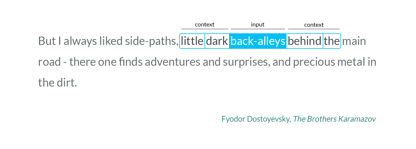
CBOW把一個詞從詞窗剔除。在CBOW下給定n詞圍繞著詞w，word2vec預測一個句子中其中一個缺漏的詞c，即以機率 P(c|w) 來表示。相反地，Skip-gram 給定詞窗中的文本，預測當前的詞 P(w|c)。

一個詞在神經網路中，原本應該是以 one-hot encoding 的方式表達。假如詞典有十萬個詞，那麼 one-hot encoding 就會用十萬維的向量表示，這顯然太大了。

使用詞向量技術，我們可以把十萬維的 one-hot 向量，轉換成 300 維的向量，這對神經網路而言，可以減小模型大小，並且讓相似詞的距離變近，相當於先對詞彙做了一個 Clustering 的動作。

你可以想像 CBOW/Skip-Grame 這些算法，會透過鄰近詞彙，將相似的詞拉近，在經過幾輪的拉扯之後，相似的詞彙就會在空間中聚集在一起了！

這個技術提出之後，在 Python 社群當中被 gensim 等套件實作出來。舉例而言，我們可以用下列程式，載入事先建構好的詞向量，然後列出和指定詞相似的詞彙 ...

import gensim.downloader
model = gensim.downloader.load('glove-twitter-25')

print(f"model.most_similar('twitter')={model.most_similar('twitter')}")
print(f"model.most_similar('dog')={model.most_similar('dog')}")
print(f"model.most_similar('mother')={model.most_similar('mother')}")
print(f"model.most_similar('king')={model.most_similar('king')}")
print(f"model.most_similar('push')={model.most_similar('push')}")
print(f"model.most_similar(positive=['woman', 'king'], negative=['man'])={model.most_similar(positive=['woman', 'king'], negative=['man'])}")

執行結果

$ python pretrained.py
[==================================================] 100.0% 104.8/104.8MB downloaded
model.most_similar('twitter')=[('facebook', 0.9480050802230835), ('tweet', 0.9403423070907593), ('fb',
0.9342359900474548), ('instagram', 0.9104824066162109), ('chat', 0.8964963555335999), ('hashtag', 0.8885936737060547), ('tweets', 0.8878158330917358), ('tl', 0.8778461217880249), ('link', 0.8778210878372192), ('internet', 0.8753897547721863)]
model.most_similar('dog')=[('cat', 0.9590820074081421), ('dogs', 0.9244232177734375), ('horse', 0.9209403395652771), ('monkey', 0.9146843552589417), ('pig', 0.9116265177726746), ('kid', 0.902455747127533),
('puppy', 0.9024085402488708), ('bear', 0.9013873934745789), ('pet', 0.8971227407455444), ('dirty', 0.8893660306930542)]
model.most_similar('mother')=[('father', 0.9509677886962891), ('child', 0.937720537185669), ('daughter', 0.9361845254898071), ('friend', 0.929322361946106), ('sister', 0.9281293153762817), ('wife', 0.9274636507034302), ('woman', 0.9214695692062378), ('girl', 0.9200195074081421), ('mom', 0.9165931940078735),
('dad', 0.9141176342964172)]
model.most_similar('king')=[('prince', 0.93374103307724), ('queen', 0.920242190361023), ('aka', 0.9176921844482422), ('lady', 0.9163240194320679), ('jack', 0.9147355556488037), ("'s", 0.9066898822784424), ('stone', 0.898237407207489), ('mr.', 0.8919408917427063), ('the', 0.889343798160553), ('star', 0.8892088532447815)]
model.most_similar('push')=[('carry', 0.9432512521743774), ('hold', 0.9204719662666321), ('step', 0.9168412685394287), ('handle', 0.9149768352508545), ('reach', 0.9070982336997986), ('take', 0.9024858474731445), ('able', 0.8978244066238403), ('moves', 0.8954479098320007), ('aim', 0.8929283022880554), ('pass', 0.8912724852561951)]
model.most_similar(positive=['woman', 'king'], negative=['man'])=[('meets', 0.8841923475265503), ('prince', 0.832163393497467), ('queen', 0.8257461786270142), ('’s', 0.817409873008728), ('crow', 0.81349939
1078949), ('hunter', 0.8131038546562195), ('father', 0.8115834593772888), ('soldier', 0.81113600730896), ('mercy', 0.8082393407821655), ('hero', 0.8082264065742493)]

從第一條 model.most_similar('twitter') 可以看到，相似詞有 facebook, tweet, fb, instgram 等等，這非常合理，因此詞向量可以有效地將相似的詞彙拉在一起。

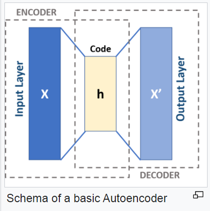
神經網路的 AutoEncoder 模型，也可以用來訓練詞向量，該模型具有 Encoder/Decoder 架構，如下圖所示：

如果我們想自己設計一個 AutoEncoder 層，那可以參考下列文章：

• Word2vec from Scratch

以下是文章中詞嵌入層的設計方法

def init_network(vocab_size, n_embedding):
    model = {
        "w1": np.random.randn(vocab_size, n_embedding),
        "w2": np.random.randn(n_embedding, vocab_size)
    }
    return model

其中 w1 是將 one-hot 向量 (vocab_size, 例如十萬維) 轉成 n_embedding 的詞向量大小 (n_embedding, 例如 300 維)

而 w2 則將 n_embedding 維度的詞向量，又轉回 vocab_size 大小。

以下程式會建構出一個 embed 層，將 vocab_size = len(word_to_id) 詞典大小的詞向量，轉為 n_embedding=10 維的詞向量。

model = init_network(len(word_to_id), 10)

這種架構，其實就是一種用來降維的 Encoder/Decoder 架構，希望解碼後的詞盡可能就是原來那個詞，但維度卻可以壓縮得很小。

def forward(model, X, return_cache=True):
    cache = {}
    
    cache["a1"] = X @ model["w1"]
    cache["a2"] = cache["a1"] @ model["w2"]
    cache["z"] = softmax(cache["a2"])
    
    if not return_cache:
        return cache["z"]
    return cache

上述程式所對應的數學公式如下：

$A_1 = X W_1$

$A_2 = A_1 W_2$

$Z = softmax(A_2)$

所以 Embedding model 是一個將vocab_size 大小的輸入， 用 W1 編碼成 n_embedding 大小的向量。

然後用 W2 將其還原，並讓最後輸出的 Z 盡可能就是原來的 one-hot encoding 的那種網路。

其 loss 的定義如下：

$\frac{\partial L}{\partial A_2} = Z-y$

上述模型的反傳遞程式碼如下

def backward(model, X, y, alpha):
    cache  = forward(model, X)
    da2 = cache["z"] - y
    dw2 = cache["a1"].T @ da2
    da1 = da2 @ model["w2"].T
    dw1 = X.T @ da1
    assert(dw2.shape == model["w2"].shape)
    assert(dw1.shape == model["w1"].shape)
    model["w1"] -= alpha * dw1
    model["w2"] -= alpha * dw2
    return cross_entropy(cache["z"], y)

上述的 backward 程式，目的是讓 z 與 y 之間的 cross_entropy 愈小愈好，也就是正確將 y 壓縮後又還原為 y 的比例愈高愈好。

以上就是《詞向量》的運作原理，希望這樣的說明，可以讓你更了解詞向量技術在《深度學習語言模型》中的地位！