twopiece: Two-Piece Distributions

• Homepage: https://github.com/quantgirluk/twopiece
• Pip Repository: twopiece
• Demo: Python Notebook

---

• Overview
• Supported Distributions
• Main Features
• Quick Start
• Install

---

Overview

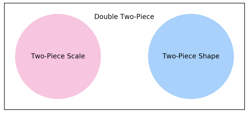
The twopiece library provides a Python implementation of the family of Two Piece distributions. It covers three subfamilies Two-Piece Scale, Two-Piece Shape, and Double Two-Piece. The following diagram shows how these families relate.

---

Two-Piece Scale

The family of two–piece scale distributions is a family of univariate three parameter location-scale models, where skewness is introduced by differing scale parameters either side of the mode.

Definition. Let $f: \mathbb{R} \mapsto \mathbb{R}_{+}$ be a unimodal symmetric (around zero) probability density function (pdf) from the location-scale family, possibly including a shape parameter $\delta$. Then, the pdf of a member of the two-piece family of distributions is given by

$$ s\left(x; \mu,\sigma_1,\sigma_2, \delta\right) = \begin{cases} \dfrac{2}{\sigma_1+\sigma_2}f\left(\dfrac{x-\mu}{\sigma_1};\delta\right), \mbox{if } x < \mu, \\ \dfrac{2}{\sigma_1+\sigma_2}f\left(\dfrac{x-\mu}{\sigma_2};\delta\right), \mbox{if } x \geq \mu. \\ \end{cases} $$

Example. If $f$ corresponds to the normal pdf, then $s$ corresponds to the pdf of the Two-Piece Normal distribution as proposed by Gustav Fechner in 1887.

---

Two-Piece Shape

The family of two–piece shape distributions is a family of univariate three parameter location-scale models, where skewness is introduced by differing shape parameters either side of the mode.

Definition. Let $f: \mathbb{R} \mapsto \mathbb{R}_{+}$ be a unimodal symmetric (around 0) probability density function (pdf) from the location-scale family which includes a shape parameter $\delta$. Then, the pdf of a member of the two-piece family of distributions is given by

$$ s\left(x; \mu,\sigma,\delta_1 \delta_2\right) = \begin{cases} \dfrac{2\epsilon}{\sigma}f\left(\dfrac{x-\mu}{\sigma};\delta_1\right), \mbox{if } x < \mu, \\ \dfrac{2(1 -\epsilon)}{\sigma}f\left(\dfrac{x-\mu}{\sigma};\delta_2\right), \mbox{if } x \geq \mu. \\ \end{cases} $$

where

$$ \epsilon = \dfrac{f(0;\delta_2)}{f(0;\delta_1)+f(0;\delta_2)}. $$

Example. If $f$ corresponds to the Student-t pdf, then $s$ corresponds to the pdf of the Two-Piece Shape Student-t distribution. Note that $s$ has different shape parameter on each side mode but the same scale.

---

Double Two-Piece

The family of double two–piece distributions is obtained by using a density–based transformation of unimodal symmetric continuous distributions with a shape parameter. The resulting distributions contain five interpretable parameters that control the mode, as well as both scale and shape in each direction.

Definition. Let $f: \mathbb{R} \mapsto \mathbb{R}_{+}$ be a unimodal symmetric (around 0) probability density function (pdf) from the location-scale family which includes a shape parameter $\delta$. Then, the pdf of a member of the two-piece family of distributions is given by

$$ s\left(x; \mu,\sigma_1,\sigma_2, \delta_1, \delta_2 \right) = \begin{cases} \dfrac{2\epsilon}{\sigma_1}f\left(\dfrac{x-\mu}{\sigma_1};\delta_1\right), \mbox{if } x < \mu, \\ \dfrac{2(1 -\epsilon)}{\sigma_2}f\left(\dfrac{x-\mu}{\sigma_2};\delta_2\right), \mbox{if } x \geq \mu. \\ \end{cases} $$

where

$$ \epsilon = \dfrac{\sigma_1f(0;\delta_2)}{\sigma_2f(0;\delta_1)+\sigma_1 f(0;\delta_2)}. $$

Example. If $f$ corresponds to the Student-t pdf then $s$ corresponds to the pdf of the Double Two-Piece Student-t distribution. Note that $s$ has different scale and shape on each side of the mode.

---

Notes

For technical details on this families of distributions we refer to the following two publications which serve as reference for our implementation.

• Inference in Two-Piece Location-Scale Models with Jeffreys Priors published in Bayesian Anal. Volume 9, Number 1 (2014), 1-22.

• Bayesian modelling of skewness and kurtosis with Two-Piece Scale and shape distributions published in Electron. J. Statist., Volume 9, Number 2 (2015), 1884-1912.

For the R implementation we refer to the following packages.

• twopiece, DTP, and TPSAS

twopiece has been developed and tested on Python 3.6, and 3.7.

---

Supported Distributions

Implementation is provided for the following distributions.

Two-Piece Scale

Name	Function	Parameters
Two-Piece Normal	tpnorm	loc, sigma1, sigma2
Two-Piece Laplace	tplaplace	loc, sigma1, sigma2
Two-Piece Cauchy	tpcauchy	loc, sigma1, sigma2
Two-Piece Logistic	tplogistic	loc, sigma1, sigma2
Two-Piece Student-t	tpstudent	loc, sigma1, sigma2, shape
Two-Piece Exponential Power	tpgennorm	loc, sigma1, sigma2, shape
Two-Piece SinhArcSinh	tpsas	loc, sigma1, sigma2, shape

Two-Piece Shape

Name	Function	Parameters
Two-Piece-Shape Student-t	tpshastudent	loc, sigma, shape1, shape2
Two-Piece-Shape Exponential Power	tpshagennorm	loc, sigma, shape1, shape2
Two-Piece-Shape SinhArcSinh	tpshasas	loc, sigma, shape1, shape2

Double Two-Piece

Name	Function	Parameters
Double Two-Piece Student-t	dtpstudent	loc, sigma1, sigma2, shape1, shape2
Double Two-Piece Exponential Power	dtpgennorm	loc, sigma1, sigma2, shape1, shape2
Double Two-Piece SinhArcSinh	dtpsinhasinh	loc, sigma1, sigma2, shape1, shape2

---

Main Features

We provide the following functionality for all the supported distributions.

Function	Method	Parameters
Probability Density Function	pdf	x
Cumulative Distribution Function	cdf	x
Quantile Function	ppf	q
Random Sample Generation	random_sample	size

---

Quick Start

Install

We recommend install twopiece using pip as follows.

pip install twopiece

To illustrate usage two-piece scale distributions we will use the two-piece Normal, and two-piece Student-t. The behaviour is analogous for the rest of the supported distributions.

---

1. Create a twopiece instance

First, we load the family (scale, shape and double) of two-piece distributions that we want to use.

from twopiece.scale import *
from twopiece.shape import *
from twopiece.double import *

To create an instance we need to specify either 3, 4, or 5 parameters:

For the Two-Piece Normal we require:

• loc: which is the location parameter
• sigma1, sigma2 : which are both scale parameters

loc=0.0
sigma1=1.0
sigma2=1.0
dist = tpnorm(loc=loc, sigma1=sigma1, sigma2=sigma2)

For the Two-Piece Student-t we require:

• loc: which is the location parameter
• sigma1, sigma2 : which are both scale parameters
• shape : which defines the degrees of freedom for the t-Student distribution

loc=0.0
sigma1=1.0
sigma2=2.0
shape=3.0
dist = tpstudent(loc=loc, sigma1=sigma1, sigma2=sigma2, shape=shape)

For the Double Two-Piece Student-t we require:

• loc: which is the location parameter
• sigma1, sigma2 : which are both scale parameters
• shape1, shape2 : which define the degrees of freedom for the t-Student distribution on each side of the mode.

loc=0.0
sigma1=1.0
sigma2=2.0
shape1=3.0
shape2=10.0
dist = dtpstudent(loc=loc, sigma1=sigma1, sigma2=sigma2, shape1=shape1, shape2=shape2)

Hereafter we assume that there is a twopiece instance called dist.

2. Evaluate and visualise the probability density function (pdf)

We can evaluate the pdf on a single point or an array type object

dist.pdf(0)

dist.pdf([0.0,0.25,0.5])

To visualise the pdf use

x = arange(-12, 12, 0.1)
y = dist.pdf(x)
plt.plot(x, y)
plt.show()

3. Evaluate the cumulative distribution function (cdf)

We can evaluate the cdf on a single point or an array type object

dist.cdf(0)

dist.cdf([0.0,0.25,0.5])

To visualise the cdf use

x = arange(-12, 12, 0.1)
y = dist.cdf(x)
plt.plot(x, y)
plt.show()

4. Evaluate the quantile function (ppf)

We can evaluate the ppf on a single point or an array type object. Note that the ppf has support on [0,1].

dist.ppf(0.95)

dist.ppf([0.5, 0.9, 0.95])

To visualise the ppf use

x = arange(0.001, 0.999, 0.01)
y = dist.ppf(x)
plt.plot(x, y)
plt.show()

5. Generate a random sample

To generate a random sample we require:

• size: which is simply the size of the sample

sample = dist.random_sample(size = 100)

---

Thanks for Visiting! ✨

Connect with me via:

• 🦜 Twitter
• 👩🏽‍💼 Linkedin
• 📸 Instagram
• 👾 Personal Website

⭐️ If you like this repository, please give it a star! ⭐️