Output figures Python
The figures generated depend on the data available.
Figures will be generated for each cluster identified that passes curation.
For all data types, Python will plot:
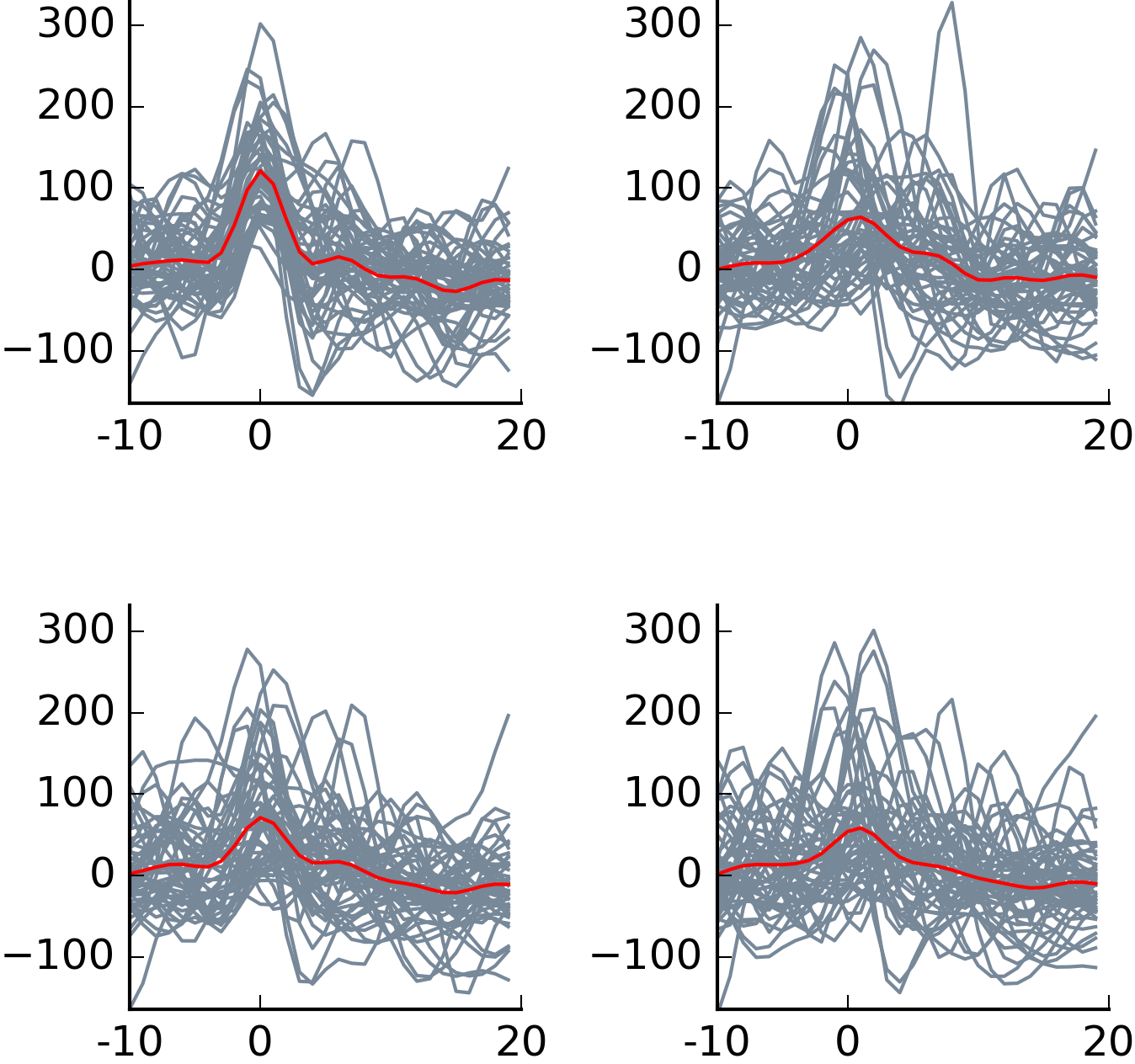
(1) Waveforms - 50 example waveforms from the cluster are plotted (grey) for each channel on the tetrode on which the event was detected, with an average waveform overlaid (red). The x axis represents number of data samples (30k/sec), and the y axis shows change in voltage in mV.
 (2) 2 autocorrelograms - the first shows time between -10 and 10 milliseconds, the second shows between -250 and 250.

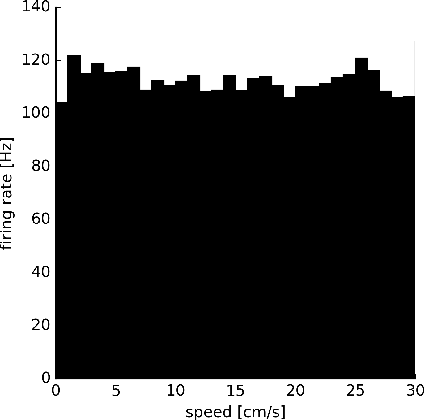
 (3) Spike histograms - plots number of spikes against sampling points in units of 1e7, and firing rate against speed of the animal in cm/s.

For open field data, uses Bonsai tracking data to plot:
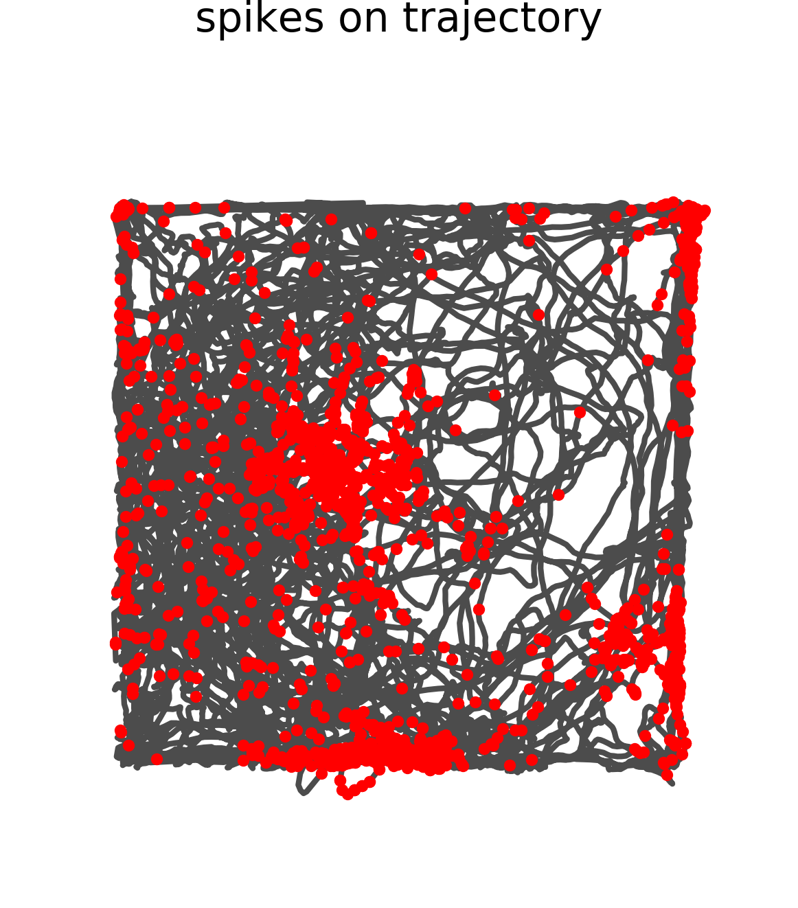
(1) Trajectory of animal (grey) with spikes overlaid (red dots).
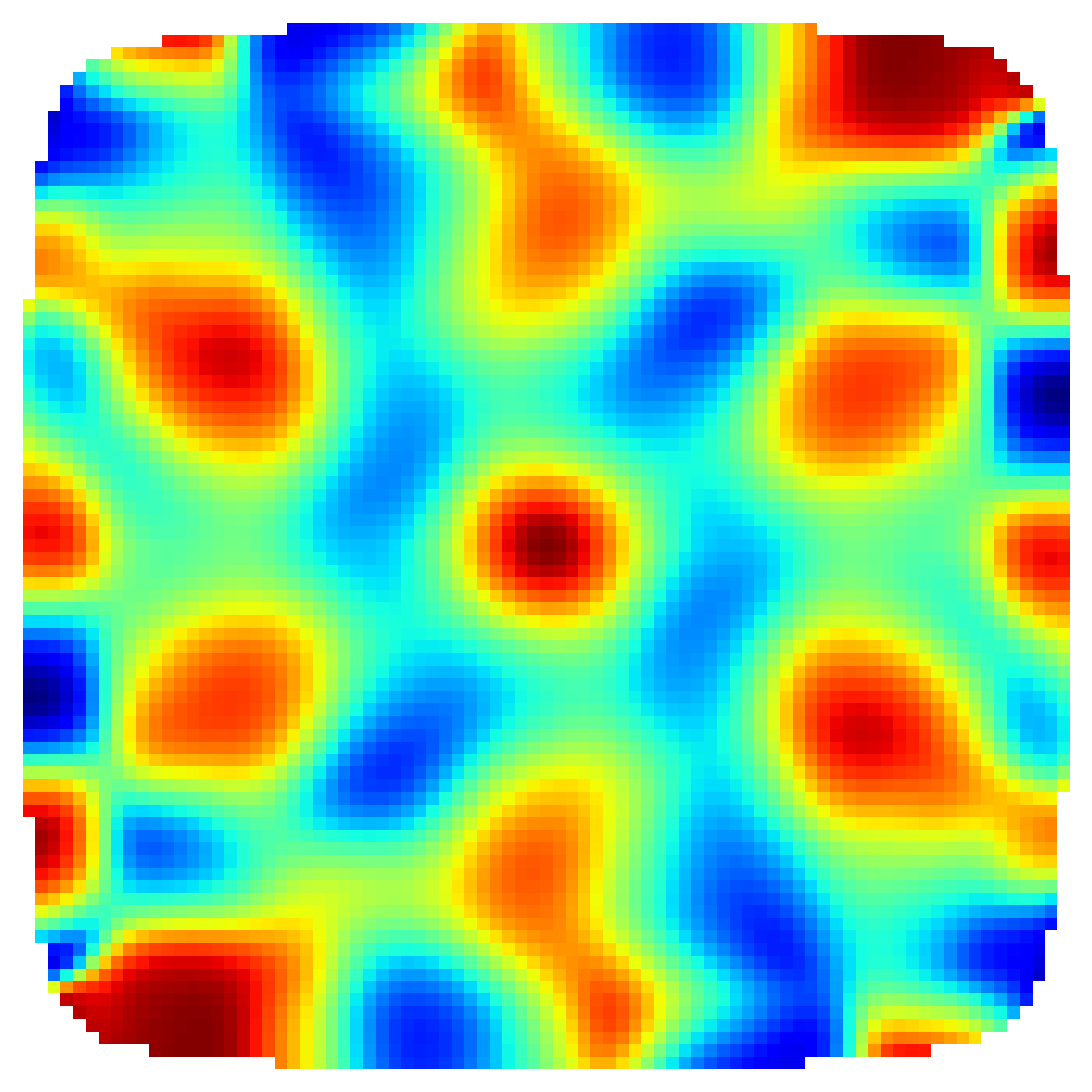
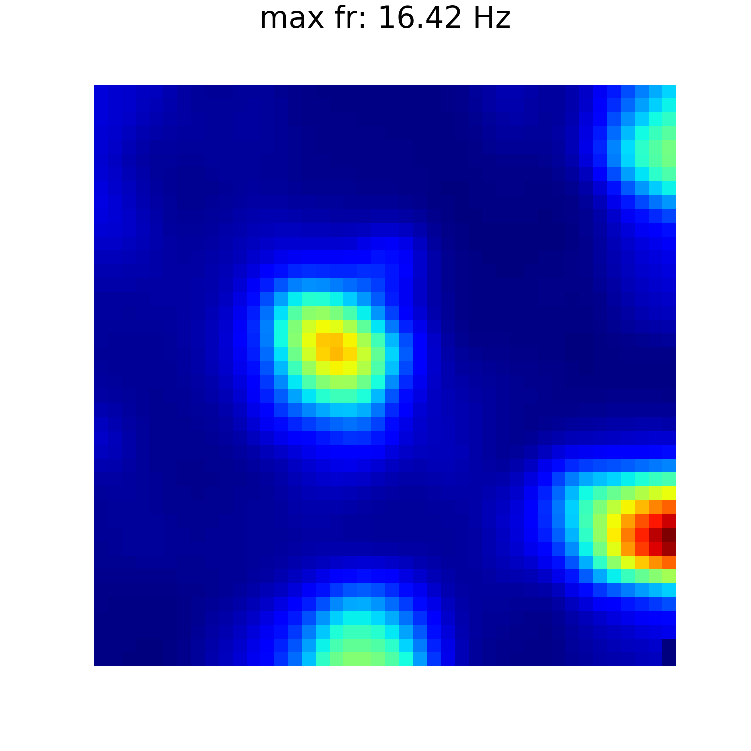
 (2) Firing rate map - shows firing rate as colour within pixels, and displays maximum firing rate.
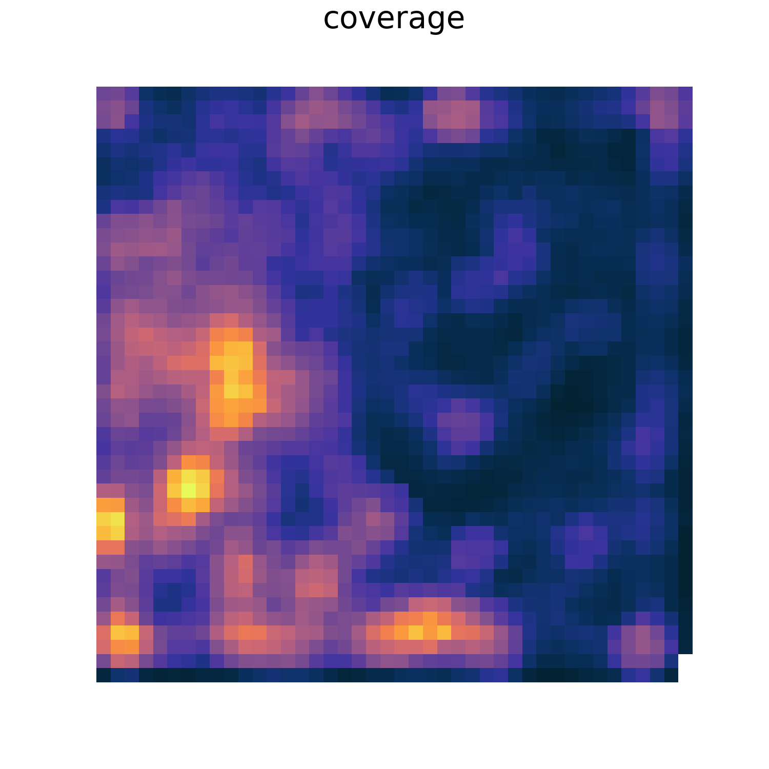
 (3) Heat map of animal's coverage of environment.
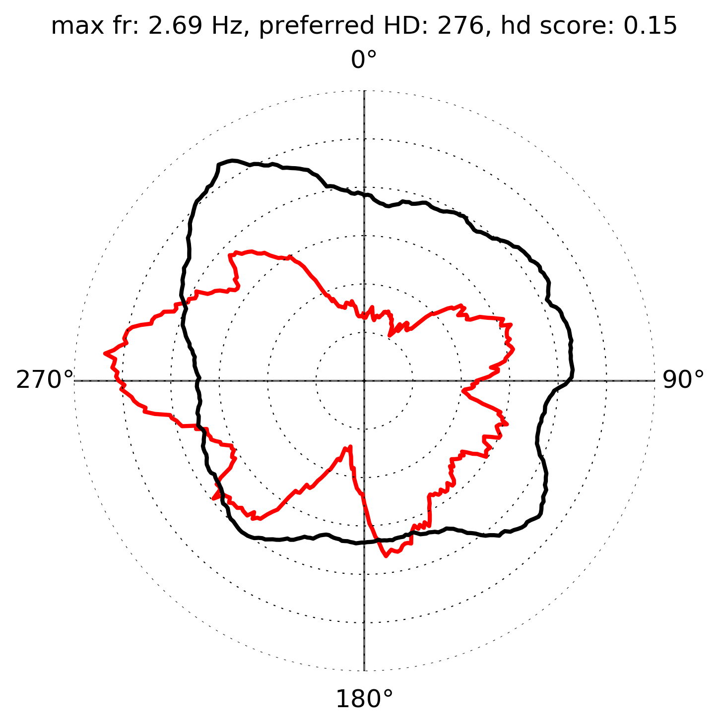
 (4) Head direction - firing rate against direction of head in degrees. Also displays maximum firing rate, preferred head direction, and head direction score.
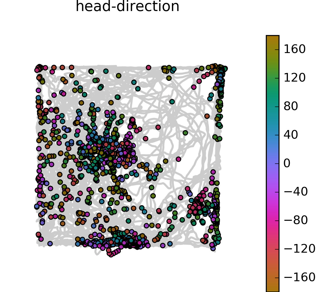
 (5) Head direction with trajectory - shows head direction (-180 to 180 degrees) as colour of spikes on trajectory plot.