GCP Data Architecture

🇧🇷 Versão em português

Document that presents a data architecture based on GCP, designed to efficiently deliver information received from multiple sources for both fast consumption and analytical use.

The solution was built to operate at scale with high data volume but can be simplified for scenarios with lower load or complexity.

1. Data Submission 🏌️‍♂️

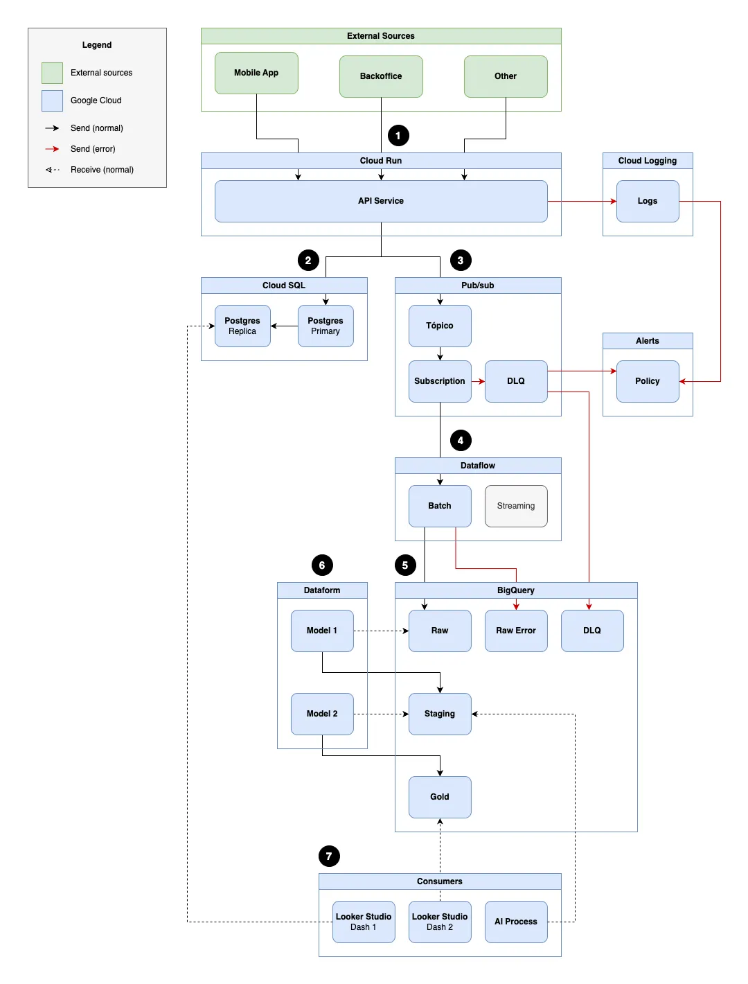
There are three external sources that write data into the solution:

• Mobile App: used by drivers (sends and consumes data)
• Backoffice: used by supervisors (sends and consumes data)
• Other: integrations or scripts (only send data)

All sources communicate with the API hosted on Cloud Run via HTTP calls following the REST pattern, using the appropriate method for each operation type:

Method	Purpose	Example
POST	Record insertion	POST /drivers
PUT	Record update	PUT /trips/123
DELETE	Record deletion	DELETE /customers/12

PUT /trips/123
Content-Type: application/json

{
  "status": "completed",
  "end_date": "2025-04-03T18:00:00Z"
}

Metadata

Each request carries metadata:

Metadata	Source	Purpose
timestamp	generated by API	For ordering and auditing
auditid	generated by API	Unique request ID used in data lifecycle
source	header or token	Identifies source (e.g., app, backoffice)
operation	HTTP method	Defines if it is insert/update/delete
entity	URL path	Defines the table/entity
userid	URL path	Identifies who generated the record

When receiving a request from any external source, the Cloud Run API performs two actions:

• Request Logging: the received content, headers, HTTP status, and response time are automatically logged in Cloud Logging, ensuring traceability.

• Data Forwarding: after initial processing, the data is forked—persisted in a relational database (used for fast reads) and published to Pub/Sub (where it is processed asynchronously).

Logs can be analyzed via Log Analytics, allowing the creation of alerts and dashboards to identify unexpected behaviors.

2. Persistence in PostgreSQL 💾

The data is processed according to business rules and saved in the PostgreSQL relational database in a primary instance using Cloud SQL.

Operational and analytical queries are performed through a replica instance, which supports reports requiring lower latency without overloading the primary instance.

If a write error occurs, the transaction is rolled back and the HTTP response reflects the failure.

3. Publishing to Pub/Sub 📬

After receiving the request, the API publishes an event to the Pub/Sub topic, and the message is delivered to the Dataflow pipeline. Pub/Sub ensures message delivery via automatic retries:

• Each message can be retried up to a maximum number of attempts (e.g., 5 times)
• The consumer must acknowledge receipt with an ack
• If it fails after retries, the message is sent to the DLQ

Messages in the DLQ

The DLQ is implemented as a secondary Pub/Sub topic, receiving messages that exceeded the retry limit for the main subscription:

• The DLQ topic is integrated with BigQuery using the native ingestion feature via Pub/Sub.
• Every message published to the DLQ is inserted into a table without requiring an additional pipeline.

{
  "timestamp": "2025-04-03T19:15:32.123Z",
  "auditid": "req-123abc",
  "userid": "abc321",
  "source": "backoffice",
  "operation": "update",
  "entity": "trips",
  "id": "abc123",
  "data": {
    "id": "abc123",
    "status": "completed",
    "end_date": "2025-04-03T18:00:00Z"
  },
  "messageid": "abc123",
  "publishtime": "2025-04-03T19:15:33.543Z"
}

4. Processing with Dataflow 🚴‍♂️

The Dataflow pipeline is responsible for consuming the events published to the Pub/Sub topic and writing them to BigQuery in the simplest form possible.

Since the flow is designed to operate in batch mode, Dataflow groups events into configurable time windows (e.g., every 5 minutes), helping to reduce costs:

• Directly reads the JSON event received from Pub/Sub
• Separates and routes events according to the entity (e.g., trips, drivers, customers)
• Persists to separate tables within the raw dataset, one for each entity
• Routes internal Dataflow errors (e.g., invalid parsing) to specific error tables in BigQuery

Designed to support flexible schemas using data:STRING type in BigQuery. This allows storing incoming data regardless of changes in the payload structure.

5. Storage in BigQuery 🗃️

raw dataset

In BigQuery, events processed by Dataflow are stored in a dataset named raw. In this dataset, each entity has its own table. This approach provides better organization, performance, and flexibility to evolve schemas independently.

• raw.trips
• raw.drivers
• raw.customers
• raw_errors.trips (for malformed events)

Expected structure for tables in raw

Column	Type	Description
timestamp	TIMESTAMP	When the data was generated
auditid	STRING	Unique request ID
userid	STRING	Unique user ID
operation	STRING	Operation type: insert, update or delete
source	STRING	Request source (app, backoffice, etc.)
id	STRING	Unique record identifier
data	STRING	Original payload sent
messageid	STRING	Unique Pub/Sub message ID
publishtime	TIMESTAMP	When the message was published to Pub/Sub
ingestiondatetime	TIMESTAMP	When the data was stored in BigQuery

Tables are partitioned by DATE(timestamp) and can be clustered by id and operation to improve query performance.

Invalid or malformed events are stored in mirrored tables in the raw_errors dataset, with the same structure.

This stage can also perform data consolidation to periodically keep only the latest version of each record, reducing storage costs.

6. Transformations with Dataform 🧞‍♂️

Dataform is responsible for organizing the data stored in the raw dataset tables, applying business rules, additional validations, and the necessary modeling to make the data ready for analysis.

Staging

In this step, each table in the raw dataset has a corresponding table in the staging dataset. These tables are updated through scheduled transformations, usually via DAGs or Dataform jobs.

These staging tables perform:

• Reading from raw data (raw.*)
• Extraction of fields from the data JSON
• Standardization of names and formats
• Removal of duplicates
• Filtering out invalid or unnecessary records

staging.trips

Column	Type	Description
id	STRING	Unique trip identifier
status	STRING	Current trip status
end_date	TIMESTAMP	Trip completion timestamp
lasttimestamp	TIMESTAMP	Timestamp of the last request that updated the record
lastuserid	STRING	Last user who updated the record
lastoperation	STRING	Last operation performed on the record
ingestiondatetime	TIMESTAMP	When the data was stored in BigQuery

config {
  type: "table",
  partition_by: "DATE(ingestiondatetime)",
  schema: "staging",
  name: "trips"
}

SELECT
  id,
  MAX_BY(data.status, timestamp) AS status,
  MAX_BY(data.end_date, timestamp) AS end_date,
  MAX(timestamp) AS lasttimestamp,
  MAX_BY(userid, timestamp) AS lastuserid,
  MAX_BY(operation, timestamp) AS lastoperation,
  CURRENT_TIMESTAMP() AS ingestiondatetime
FROM raw.trips
GROUP BY id

This table is partitioned by DATE(ingestiondatetime) to improve read performance and reduce analytical query costs.

By default, we use MAX_BY(field, timestamp) to reconstruct the complete state of a record from partial events. This ensures each field shows the most recent value, even when updates arrive at different times and include only part of the data.

Gold

This layer represents data ready for consumption by BI tools like Looker Studio. Models are built from the staging tables, usually through scheduled jobs in Dataform. This layer often contains enriched, validated, and organized data tailored to visualization and reporting needs.

gold.driver_issues_24h

Column	Type	Description
driver_name	STRING	Driver's full name
driver_phone	STRING	Driver's contact phone
issue_name	STRING	Identified issue type
issue_garage	STRING	Garage name linked to the issue
issue_garage_contact	STRING	Contact for the garage handling the issue
issue_timestamp	TIMESTAMP	Timestamp when the issue was recorded

config {
  type: "table",
  schema: "gold",
  name: "driver_issues_24h",
  partition_by: "DATE(issue_timestamp)"
}

WITH recent_issues AS (
  SELECT
    issue_id,
    driver_id,
    issue_timestamp
  FROM staging.driver_issues
  WHERE issue_timestamp >= TIMESTAMP_SUB(CURRENT_TIMESTAMP(), INTERVAL 24 HOUR) and operation <> 'delete'
)

SELECT
  d.name AS driver_name,
  d.phone AS driver_phone,
  i.name AS issue_name,
  i.garage AS issue_garage,
  i.garage_contact AS issue_garage_contact,
  ri.issue_timestamp
FROM recent_issues AS ri
LEFT JOIN staging.drivers AS d ON ri.driver_id = d.id
LEFT JOIN staging.issues AS i ON ri.issue_id = i.id

This table is regenerated once a day, but incremental loading strategies could be used to maintain history (e.g., loading from the latest counter).

7. Data Consumption 🍫

After transformation and modeling in the staging and gold layers, data is ready for consumption through different channels depending on application or business needs.

Looker Studio

Looker Studio can connect to both BigQuery and PostgreSQL (replica). Source selection depends on data type and latency requirements:

• When connected to BigQuery, it can leverage caching mechanisms to avoid new job creation at each access and reduce response time.
• When connected to the PostgreSQL replica, Looker Studio allows lower latency queries—ideal for operational or near real-time dashboards.

Analytical processes and AI models

Data in the staging and gold layers can also be used as input for:

• Machine learning model training
• Analytical batch routines
• Operational forecasts

Notes ✍️

Data Steps

• It is possible to track the data journey from the request to its insertion in BigQuery, in the raw layer, using the auditid.

• It is also possible to verify which data was successfully sent to Pub/Sub and reached the BigQuery raw layer.

• The timestamps for each step can be followed using the request timestamp, the Pub/Sub publish time publishtime, and the ingestion time in BigQuery via ingestiondatetime.

• The history of each event can be stored for a specific period, and later, a Scheduled Query can be run to consolidate and retain only the latest version of each record, both in the raw and staging layers, to reduce costs.

Costs

• Although not the most user-friendly tool, Google provides a pricing calculator to help estimate costs. You can also check the documentation for each resource used.

• More specific analysis can also help reduce costs. For example, understanding whether your data will be stored as logical or physical storage in BigQuery (more details).

Sophistication

• You can create a Cloud Run service and connect it to BigQuery to be triggered during query execution (more details), enabling use cases like notifying drivers through alerts.

• You can also create a federated connection in BigQuery to access relational databases (more details), enriching reports with live data.

Adaptations

• In step 2, if data is not submitted frequently, the Cloud SQL replica can be omitted.

• Steps 3 and 4 can be removed if data is written directly to BigQuery using the BigQuery Write API from Cloud Run.

• Step 4 can also be skipped by using direct Pub/Sub to BigQuery integration (more details).

• If Dataform is too heavy for your context, it can be replaced by Scheduled Queries.

Improvements

• The proposed architecture is designed for educational purposes and can be customized based on the context and data volume of each application.

---

Made with ❤️ in Curitiba 🌳 ☔️