0- Introduction and course overview (Levine (L), Finn (F), Schulman (S)):
-
L: Course information and todos:
- Overall the course will cover:
- supervised learning to decision making
- Basic RL: Q-Learning and Policy gradients
- Advanced model learning, prediction, distillation, reward learning.
- DeepRL: Trust Region Policy, Actor-Critic Methods, Exploration
- Open Problems
- HW:
- HW1: Imitation Learning (Control via supervised learning)
- HW2: Basic (Sh) RL
- HW3: Deep Q-Learning:
- HW4: Deep Policy grads
- HW5: Final Project (Research)
- Using more sensory information form environment can allow the agent to navigate better towards reward and explore.
- Hence, the need for vision, audio and other sensory inputs.
- Problem: How do we process all these information coming from the sensory inputs?
- Answer: Deep in the Deep Learning, using neural networks and function approximation to process complex inputs into the RL algorithm which can choose an action.
- Let's be clear here:
- Deep Learning for processing the complex information
- RL to select the next action using processed inputs by NNs
- Interesting work: Reinforcement learning in the brain - Yael Niv
- Sutton and Barto (1990) suggested the temporal difference learning rule as a model of prediction learning in Pavlovian conditioning.
- Basal ganglia appears to be related to reward system
- What can deep learning and RL do well now?
- high degree of proficiency in domains with known rules.
- learn skills with low sensory info, but a lot of repetition.
- learning from human imitation.
- The Hard things:
- Humans (we) can learn real quick! VS RL is usually slow.
- Humans (we) can reuse previous information! VS Transfer learning in deep RL is an open problem.
- Not clear what the reward function is.
- Not clear what the role of prediction should be.
- Turing said: Why try rebuilding an adult brain? Try simulating a child's one. (Hence the shitty robo-cops falling into water fountains)
- Overall the course will cover:
-
F: Beyond learning rewards
- child's play vs rl agent in an environment. (In the real world, humans don’t get a score.)
- reward funcs are essential to the structure the problem as RL.
- real-world domains: reward/cost often difficult to specify:
- robotic manipulation
- autonomous driving
- dialog systems
- virtual assistants
- ...
- real-world domains: reward/cost often difficult to specify:
- List all the forms of supervision?
- imitation: autonomous-cars
- inferring intentions:
- Inverse RL: demonstrations
- Inverse RL: learned behavior
- Inverse RL: demonstrations
- inferring intentions:
- model-based, self-supervision: (Behavior via Prediction)
- auxiliary tasks:
- Sources of Auxiliary Supervision:
- touch, audio, depth)
- learning multiple, related tasks
- task-relevant properties of the world
- imitation: autonomous-cars
-
S: RL is a branch of ML that concerns about taking sequences of actions.
- Formalized as partially observable Markov decision process (POMDP)
- Observations, Actions, Rewards (this can be applied to real-world stuff, as in Business Operations)
- O: current levels / score
- A: number of steps to make / purchase
- R: profit / reheal or something to continue
- Other ML problems falling into this realm:
- Classification with Hard Attention
- Sequential/structured prediction, e.g., machine translation
- Deep Reinforcement Learning = RL learning using NNs to ~~~ functions.
- Policies (next actions)
- Value Funcs (measure how good state actions-pairs are)
- Dynamic Models (predict next states and rewards)
- Supervised learning:
- Contextual bandits:
- In RL vs other ML areas:
- we don't have access to the full information.
- we also have to be careful, because next step is dependent on the current step taken, or current one depends on previous Xt-1. X for actions, t for Time.
- TD-backgammon yester-era
- Atari DeepQ, policy gradients, DAgger
- policy search
- AlphaGo: supervised learning + policy gradients + value functions + Monte-Carlo tree search
1- Supervised learning and decision making (L):
- Supervised Learning of Behaviors: Deep Learning, Dynamical Systems, and Behavior Cloning:
- notations: (aka notation for the elements of RL)
-
Xt: state
-
Ot: observations
-
Ut: action
-
Pi = π(Ut|Ot) - Policy
-
c(Xt,Ut) - cost function
-
r(Xt,Ut) - reward function
-
Note (those letters should be lower-case and the "t"s should be a subscript, representing TIME)
-

-

- Imitation Learning,
- Examples:
- i.e: Driving: My-Code Nvidia's example
- we can structure the problem in this format:
- Image > [Ut,Ot] >> training data >>> supervised learning to match Image + Action (Left or Right) >>>>> π(Ut|Ot) Learned
- There is an inherent flaw with this process, since the expected trajectory and the real trajectory will part away, it deviates from where it should be. Hence the car driving of the cliff.
- It only sees expert level and it will fail at edge cases.
- We can predict this from Dynamical Systems intuition.
- How can we fix this? (Nvidia's case)

- They stitch multiple cameras to each other?
- The policy alone does not know how to fix mistakes, due to this it deviates from the working trajectory. However, if we have a distribution of the trajectories and we pick from those trajectories, then we can have a stable trajectory.
- Augmenting the data by left and right.
- Or using Optimal Control for correction.
- p(x1,u1,x2,u2.....) p(†) or Gaussian Dist is obtained from iterative LQR.
- Image > [Ut,Ot] >> training data >>> supervised learning to match Image + Action (Left or Right) >>>>> π(Ut|Ot) Learned
- Learning from a stabilizing controller (deep-neuro env)
- Examples:

- One of the problems discussed is the trajectory for pData(Ot) is not necessarily close to pπø(Ot) (due to where the data comes from).
- This is a root cause of the supervised learning, where we assume the training sample and testing sample data have similar distribution.
- Question! Can we make pData(Ot) = pπø(Ot) ?
- Somewhat YES!
- DAgger (Dataset Aggregation)
- This is an algorithm that can change the pData distribution to be close enough in Test/Train.
- By running the Policy,
- then DAgger will need to obtain the labels
- run the πø to get the dataset.
- ask a human to see if it's a good action done by Policy + DAgger collector.
- lastly, aggregate; new + human label.
- This works because eventually our data comes from the Policy and regulated.
- Case study 1: trail following as classification
- Case study 2: DAgger & domain adaptation
- Case study 3: Imitation with LSTMs
- This is an algorithm that can change the pData distribution to be close enough in Test/Train.
- Other imitation learning:
-
Structured prediction
-
Interaction & active learning
-
Inverse reinforcement learning
- figure out the goal
-
cost function -> imitation?
-
The trouble with cost & reward functions
-
make sure you understood:
- Notation
- basic imitation learning algorithms; their strengths & weaknesses
2- Optimal Control, Trajectory Optimization, and Planning (L):
-
What's up?
- Previously on this course: imitation learning from a human teacher.
- Right Now: can the machine make its own decisions?
- How can we choose actions under perfect knowledge of the system dynamics?
- eg:
- A couple of Optimizations and Goals:
- Optimal control:
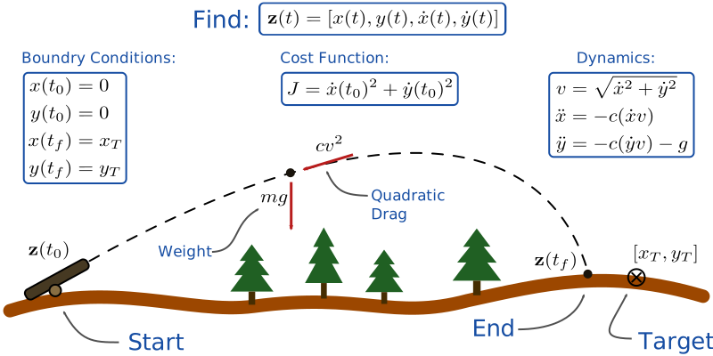
- Trajectory Optimization: back-propagation through dynamical systems
- Shooting methods vs collocation
- eg: Source: Gradient-Based Trajectory Optimization: "Trajectory optimization refers to the problem of perturbing the trajectory while satisfying all constraints so that its quality can be improved." Since I'm from Iraq, this is the best example I could understand:
- Cannon Example
- arxiv
- More useful stuff here MatthewPeterKelly - dscTutorials
- Planning: (not found here, next lec)
- How can we choose actions under perfect knowledge of the system dynamics?
- Next On this course: how can we learn unknown dynamics?
- ALSO while you're at it ask: (How can we then also learn policies? (e.g. by imitating optimal control))
-
All trajectory methods can either be described as shooting methods or collocation methods:
- The key difference is that Shooting methods use explicit integration schemes whereas collocation uses implicit.
-
Big Question: How do we make decision under known dynamics?
- often differentiate and back-prop and optimize
- keep in mind the 2nd order method helps in above step (google it if you need 34 page proof)
-
Important equation:
- Linear Case (LQR):

- Linear Case (LQR):
-
Examples of Trajectory optimization:
- Example 1: nonlinear model-predictive control (synthesis and stabilization of complex behaviors through online trajectory)
- observe the state xt
- it utilizes the iLQR to optimize plan minimize cost(xt,ut)
- execute action ut (discardut+1....ut+T)
- Example Discrete case: Monte Carlo tree search (MCTS)
- from random policy to choose rarely visited branches with best reward.
- Example 2: imitation learning from MCTS:
- same same, but aggregate at the last step, agg of the D = {o1,u1....} Which is domain data, aka human data doing stuff for imitation, i.e: the example of DAgger (i think).
- Example 1: nonlinear model-predictive control (synthesis and stabilization of complex behaviors through online trajectory)

- Linear dynamics: linear-quadratic regulator (LQR)
- The iterative Linear Quadratic Regulator algorithm ( The gist of it was at every time step linearize the dynamics, quadratize (it could be a word) the cost function around the current point in state space and compute your feedback gain off of that, as though the dynamics were both linear and consistent (i.e. didn’t change in different states). And that was pretty cool because you didn’t need all the equations of motion and inertia matrices etc to generate a control signal. You could just use the simulation you had, sample it a bunch to estimate the dynamics and value function, and go off of that.)
- The LQR, however, operates with maverick disregard for changes in the future. Careless of the consequences, it optimizes assuming the linear dynamics approximated at the current time step hold for all time. It would be really great to have an algorithm that was able to plan out and optimize a sequence, mindful of the changing dynamics of the system.
- This is exactly the iterative Linear Quadratic Regulator method (iLQR) was designed for. iLQR is an extension of LQR control, and the idea here is basically to optimize a whole control sequence rather than just the control signal for the current point in time. The basic flow of the algorithm is source
-
More on(trajectory stabilization and iterative linear quadratic regulator)....Lecture
-
Nonlinear dynamics: differential dynamic programming (DDP) & iterative LQR
-
Discrete systems: Monte-Carlo tree search (MCTS)
-
make sure you understood:
- Understand the terminology and formalisms of optimal control
- Understand some standard optimal control & planning algorithms
3- Learning Dynamical System Models from Data(L) [Week 3, Lecture 1]:
-
What's up?
-
Previously x 1 on this course: learning to act by imitating a human
-
Previously x 2 on this course: choose good actions autonomously by back-propagating (or planning) through known system dynamics (e.g. known physics)
-
Right Now: what do we do if the dynamics are unknown?
- Fitting global dynamics models (“model-based RL”)
- Fitting local dynamics models
- A couple of Optimizations and Goals:
-
Next On this course: putting it all together to learn to “imitate” without a human (e.g. by imitating optimal control), so that we can train deep network policies autonomously
-
-
learning the dynamics model right now, right here, in this lecture once for all:
- Global models and local models
- Learning with local models and trust regions
-
make sure you understood:
- formalism of model-based RL
- options for models we can use in model-based RL
- practical considerations of model learning
4- Learning Policies by Imitating Optimal Control(L):
-
HW1 is out
-
make sure you understood: * how to train policies using optimal control * tradeoffs between various methods
5- Direct Collocation Methods for Trajectory Optimization and Policy Learning (Igor) guest:
- Applied advice about the previous work.